2. Usage
2.1. Python usage
First run python or ipython REPL and try to import the project to check its version:
>>> import wltp

>>> wltp.__version__            ## Check version once more.
'1.1.0.dev0'

>>> wltp.__file__               ## To check where it was installed.
/usr/local/lib/site-package/wltp-...
If everything works, create the datamodel of the experiment. You can assemble the model-tree by the use of:
sequences,
dictionaries,
pandas.Series, andURI-references to other model-trees.
For instance:
>>> from wltp import datamodel
>>> from wltp.experiment import Experiment

>>> mdl = {
...     "unladen_mass": 1430,
...     "test_mass":    1500,
...     "v_max":        195,
...     "p_rated":      100,
...     "n_rated":      5450,
...     "n_idle":       950,
...     "n_min":        None,                           ## Manufacturers my override it
...     "n2v_ratios":         [120.5, 75, 50, 43, 37, 32],
...     "f0":   100,
...     "f1":   0.5,
...     "f2":   0.04,
... }
>>> mdl = datamodel.upd_default_load_curve(mdl)                   ## need some WOT
For information on the accepted model-data, check the code:Schemas:
>>> from wltp import utils
>>> utils.yaml_dumps(datamodel.model_schema(), indent=2)
$schema: http://json-schema.org/draft-07/schema#
$id: /wltc
title: WLTC data
type: object
additionalProperties: false
required:
- classes
properties:
classes:
...
You then have to feed this model-tree to the Experiment
constructor. Internally the pandalone.pandel.Pandel resolves URIs, fills-in default values and
validates the data based on the project’s pre-defined JSON-schema:
>>> processor = Experiment(mdl) ## Fills-in defaults and Validates model.
Assuming validation passes without errors, you can now inspect the defaulted-model before running the experiment:
>>> mdl = processor.model               ## Returns the validated model with filled-in defaults.
>>> sorted(mdl)                         ## The "defaulted" model now includes the `params` branch.
['driver_mass', 'f0', 'f1', 'f2', 'f_dsc_decimals', 'f_dsc_threshold', 'f_inertial',
 'f_n_clutch_gear2', 'f_n_min', 'f_n_min_gear2', 'f_running_threshold', 'f_safety_margin',
 'f_up_threshold', 'n2v_ratios', 'n_idle', 'n_min_drive1', 'n_min_drive2', 'n_min_drive2_stopdecel',
 'n_min_drive2_up', 'n_min_drive_down', 'n_min_drive_down_start', 'n_min_drive_set',
 'n_min_drive_up', 'n_min_drive_up_start', 'n_rated', 'p_rated', 't_cold_end', 'test_mass',
 'unladen_mass', 'v_cap', 'v_max', 'v_stopped_threshold', 'wltc_data', 'wot']
Now you can run the experiment:
>>> mdl = processor.run()               ## Runs experiment and augments the model with results.
>>> sorted(mdl)                         ## Print the top-branches of the "augmented" model.
[`cycle`, 'driver_mass', 'f0', 'f1', 'f2', `f_dsc`, 'f_dsc_decimals', `f_dsc_raw`,
 'f_dsc_threshold', 'f_inertial', 'f_n_clutch_gear2', 'f_n_min', 'f_n_min_gear2',
 'f_running_threshold', 'f_safety_margin', 'f_up_threshold', `g_vmax`, `is_n_lim_vmax`,
 'n2v_ratios', `n95_high`, `n95_low`, 'n_idle', `n_max`, `n_max1`, `n_max2`, `n_max3`,
 'n_min_drive1', 'n_min_drive2', 'n_min_drive2_stopdecel', 'n_min_drive2_up', 'n_min_drive_down',
 'n_min_drive_down_start', 'n_min_drive_set', 'n_min_drive_up', 'n_min_drive_up_start',
 'n_rated', `n_vmax`, 'p_rated', `pmr`, 't_cold_end', 'test_mass', 'unladen_mass', 'v_cap',
 'v_max', 'v_stopped_threshold', `wltc_class`, 'wltc_data', 'wot', `wots_vmax`]
To access the time-based cycle-results it is better to use a pandas.DataFrame:
>>> import pandas as pd, wltp.cycler as cycler, wltp.io as wio
>>> df = pd.DataFrame(mdl['cycle']); df.index.name = 't'
>>> df.shape                            ## ROWS(time-steps) X COLUMNS.
(1801, 107)
>>> wio.flatten_columns(df.columns)
['t', 'V_cycle', 'v_target', 'a', 'phase_1', 'phase_2', 'phase_3', 'phase_4', 'accel_raw',
 'run', 'stop', 'accel', 'cruise', 'decel', 'initaccel', 'stopdecel', 'up', 'p_inert', 'n/g1',
 'n/g2', 'n/g3', 'n/g4', 'n/g5', 'n/g6', 'n_norm/g1', 'n_norm/g2', 'n_norm/g3', 'n_norm/g4',
 'n_norm/g5', 'n_norm/g6', 'p/g1', 'p/g2', 'p/g3', 'p/g4', 'p/g5', 'p/g6', 'p_avail/g1',
 'p_avail/g2', 'p_avail/g3', 'p_avail/g4', 'p_avail/g5', 'p_avail/g6', 'p_avail_stable/g1',
 'p_avail_stable/g2', 'p_avail_stable/g3', 'p_avail_stable/g4', 'p_avail_stable/g5',
 'p_avail_stable/g6', 'p_norm/g1', 'p_norm/g2', 'p_norm/g3', 'p_norm/g4', 'p_norm/g5',
 'p_norm/g6', 'p_resist', 'p_req', 'P_remain/g1', 'P_remain/g2', 'P_remain/g3',
 'P_remain/g4', 'P_remain/g5', 'P_remain/g6', 'ok_p/g3', 'ok_p/g4', 'ok_p/g5', 'ok_p/g6',
 'ok_gear0/g0', 'ok_max_n/g1', 'ok_max_n/g2', 'ok_max_n/g3', 'ok_max_n/g4', 'ok_max_n/g5',
 'ok_max_n/g6', 'ok_min_n_g1/g1', 'ok_min_n_g1_initaccel/g1', 'ok_min_n_g2/g2',
 'ok_min_n_g2_stopdecel/g2', 'ok_min_n_g3plus_dns/g3', 'ok_min_n_g3plus_dns/g4',
 'ok_min_n_g3plus_dns/g5', 'ok_min_n_g3plus_dns/g6', 'ok_min_n_g3plus_ups/g3',
 'ok_min_n_g3plus_ups/g4', 'ok_min_n_g3plus_ups/g5', 'ok_min_n_g3plus_ups/g6', 'ok_n/g1',
 'ok_n/g2', 'ok_n/g3', 'ok_n/g4', 'ok_n/g5', 'ok_n/g6', 'ok_gear/g0', 'ok_gear/g1',
 'ok_gear/g2', 'ok_gear/g3', 'ok_gear/g4', 'ok_gear/g5', 'ok_gear/g6', 'G_scala/g0', 'G_scala/g1',
 'G_scala/g2', 'G_scala/g3', 'G_scala/g4', 'G_scala/g5', 'G_scala/g6', 'g_min', 'g_max0']
>>> 'Mean engine_speed: %s' % df.n.mean()
'Mean engine_speed: 1908.9266796224322'
>>> df.describe()
           v_class     v_target  ...     rpm_norm       v_real
count  1801.000000  1801.000000  ...  1801.000000  1801.000000
mean     46.361410    46.361410  ...     0.209621    50.235126
std      36.107745    36.107745  ...     0.192395    32.317776
min       0.000000     0.000000  ...    -0.205756     0.200000
25%      17.700000    17.700000  ...     0.083889    28.100000
50%      41.300000    41.300000  ...     0.167778    41.300000
75%      69.100000    69.100000  ...     0.285556    69.100000
max     131.300000   131.300000  ...     0.722578   131.300000

[8 rows x 10 columns]

>>> processor.driveability_report()
...
  12: (a: X-->0)
  13: g1: Revolutions too low!
  14: g1: Revolutions too low!
...
  30: (b2(2): 5-->4)
...
  38: (c1: 4-->3)
  39: (c1: 4-->3)
  40: Rule e or g missed downshift(40: 4-->3) in acceleration?
...
  42: Rule e or g missed downshift(42: 3-->2) in acceleration?
...
You can export the cycle-run results in a CSV-file with the following pandas command:
>>> df.to_csv('cycle.csv') # doctest: +SKIP
For more examples, download the sources and check the test-cases
found under the /tests/ folder.
2.2. Cmd-line usage
Warning
Not implemented in yet.
The command-line usage below requires the Python environment to be installed, and provides for executing an experiment directly from the OS’s shell (i.e. cmd in windows or bash in POSIX), and in a single command. To have precise control over the inputs and outputs (i.e. experiments in a “batch” and/or in a design of experiments) you have to run the experiments using the API python, as explained below.
The entry-point script is called wltp, and it must have been placed in your PATH
during installation. This script can construct a model by reading input-data
from multiple files and/or overriding specific single-value items. Conversely,
it can output multiple parts of the resulting-model into files.
To get help for this script, use the following commands:
$ wltp --help                               ## to get generic help for cmd-line syntax
$ wltcmdp.py -M vehicle/full_load_curve     ## to get help for specific model-paths
and then, assuming vehicle.csv is a CSV file with the vehicle parameters
for which you want to override the n_idle only, run the following:
$ wltp -v \
    -I vehicle.csv file_frmt=SERIES model_path=params header@=None \
    -m vehicle/n_idle:=850 \
    -O cycle.csv model_path=cycle
2.3. Excel usage
Attention
OUTDATED!!! Excel-integration requires Python 3 and Windows or OS X!
In Windows and OS X you may utilize the excellent xlwings library to use Excel files for providing input and output to the experiment.
To create the necessary template-files in your current-directory you should enter:
$ wltp --excel
You could type instead wltp --excel file_path to specify a different destination path.
In windows/OS X you can type wltp --excelrun and the files will be created in your home-directory
and the excel will open them in one-shot.
All the above commands creates two files:
wltp_excel_runner.xlsmThe python-enabled excel-file where input and output data are written, as seen in the screenshot below:
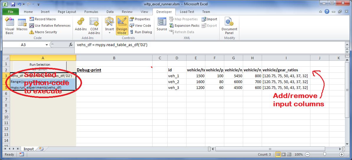
After opening it the first tie, enable the macros on the workbook, select the python-code at the left and click the button; one sheet per vehicle should be created.
The excel-file contains additionally appropriate VBA modules allowing you to invoke Python code present in selected cells with a click of a button, and python-functions declared in the python-script, below, using the
mypynamespace.To add more input-columns, you need to set as column Headers the json-pointers path of the desired model item (see Python usage below,).
wltp_excel_runner.pyUtility python functions used by the above xls-file for running a batch of experiments.
The particular functions included reads multiple vehicles from the input table with various vehicle characteristics and/or experiment parameters, and then it adds a new worksheet containing the cycle-run of each vehicle . Of course you can edit it to further fit your needs.
Note
You may reverse the procedure described above and run the python-script instead. The script will open the excel-file, run the experiments and add the new sheets, but in case any errors occur, this time you can debug them, if you had executed the script through LiClipse, or IPython!
Some general notes regarding the python-code from excel-cells:
On each invocation, the predefined VBA module
pandalonexecutes a dynamically generated python-script file in the same folder where the excel-file resides, which, among others, imports the “sister” python-script file. You can read & modify the sister python-script to import libraries such as ‘numpy’ and ‘pandas’, or pre-define utility python functions.The name of the sister python-script is automatically calculated from the name of the Excel-file, and it must be valid as a python module-name. Therefore do not use non-alphanumeric characters such as spaces(``
), dashes(-) and dots(.``) on the Excel-file.On errors, a log-file is written in the same folder where the excel-file resides, for as long as the message-box is visible, and it is deleted automatically after you click ‘ok’!