6. Cycles & Phasings
:
6.1. Cycles
The WLTC-profiles for the various classes were generated from the tables
of the specs above using the devtools/csvcolumns8to2.py script, but it still requires
an intermediate manual step involving a spreadsheet to copy the table into ands save them as CSV.
6.1.1. Phases (the problem)
6.1.1.1. GTR’s “V” phasings
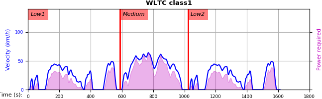
The GTR’s velocity traces have overlapping split-time values, i.e. belonging to 2 phases, and e.g. for class1 these are the sample-values @ times 589 & 1022:
class1 |
phase-1 |
phase-2 |
phase-3 |
cycle |
|---|---|---|---|---|
Boundaries |
[0, 589] |
[589, 1022] |
[1022, 1611] |
[0, 1611] |
Duration |
589 |
433 |
589 |
1611 |
# of samples |
590 |
434 |
590 |
1612 |
6.1.1.2. “Semi-VA” phasings
Some programs and most spreadsheets do not handle overlapping split-time values like that (i.e. keeping a separate column for each class-phase), and assign split-times either to the earlier or the later phase, distorting thus the duration & number of time samples some phases contain!
For instance, Access-DB tables assign split-times on the lower parts, distorting the start-times & durations for all phases except the 1st one (deviations from GTR in bold):
class1 |
phase-1 |
phase-2 |
phase-3 |
cycle |
|---|---|---|---|---|
Boundaries |
[0, 589] |
[590, 1022] |
[1023, 1611] |
[0, 1611] |
Duration |
589 |
432 |
588 |
1611 |
# of samples |
590 |
433 |
589 |
1612 |
Note
The algorithms contained in Access DB are carefully crafted to do the right thing.
The inverse distortion (assigning split-times on the higher parts) would preserve phase starting times (hint: downscaling algorithm depends on those absolute timings being precisely correct):
class1 |
phase-1 |
phase-2 |
phase-3 |
cycle |
|---|---|---|---|---|
Boundaries |
[0, 588] |
[589, 1021] |
[1022, 1611] |
[0, 1611] |
Duration |
588 |
432 |
589 |
1611 |
# of samples |
589 |
433 |
590 |
1612 |
6.1.1.3. “VA” phasings
On a related issue, GTR’s formula for Acceleration (Annex 1 3.1) produces one less value than the number of velocity samples (like the majority of the distorted phases above). GTR prescribes to (optionally) append and extra A=0 sample at the end, to equalize Acceleration & Velocities lengths, but that is not totally ok (hint: mean Acceleration values do not add up like mean-Velocities do, see next point about averaging).
Since most calculated and measured quantities (like cycle Power) are tied to the acceleration, we could refrain from adding the extra 0, and leave all phases with -1 samples, without any overlapping split-times:
class1 |
phase-1 |
phase-2 |
phase-3 |
cycle |
|---|---|---|---|---|
Boundaries |
[0, 588] |
[589, 1021] |
[1022, 1610] |
[0, 1610] |
Duration |
588 |
432 |
588 |
1610 |
# of samples |
589 |
433 |
589 |
1611 |
Actually this is “semi-VA0” phasings, above, with the last part equally distorted by -1 @ 1610. But now the whole cycle has (disturbingly) -1 # of samples & duration:
We can resolve this, conceptually, by assuming that each Acceleration-dependent sample signifies a time-duration, so that although the # of samples are still -1, the phase & cycle durations (in sec) are as expected:
class1 |
phase-1 |
phase-2 |
phase-3 |
cycle |
|---|---|---|---|---|
Boundaries |
[0, 589 ) |
[589, 1022 ) |
[1022, 1611 ) |
[0, 1611 ) |
Duration |
589 |
433 |
589 |
1611 |
# of samples |
589 |
433 |
589 |
1611 |
Summarizing the last “VA0+” phasing scheme:
each step signifies a “duration” of 1 sec,
the duration of the final sample @ 1610 reaches just before 1611sec,
# of samples for all phases are symmetrically -1 compared to Velocity phases,
it is valid for Acceleration-dependent quantities only,
it is valid for any sampling frequency (not just 1Hz),
respects the Dijkstra counting (notice the parenthesis signifying open right intervals, in the above table), BUT …
Velocity-related quantities cannot utilize this phasing scheme, must stick to the original, with overlapping split-times.
6.1.1.4. Averaging over phases
Calculating mean values for Acceleration-related quantities produce correct results only with non-overlapping split-times.
It’s easier to demonstrate the issues with a hypothetical 4-sec cycle, composed of 2 symmetrical ramp-up/ramp-down 2-sec phases (the “blue” line in the plot, below):
t |
V-phase1 |
V-phase2 |
V |
Distance |
VA-phase |
A |
|---|---|---|---|---|---|---|
[sec] |
[kmh] |
[m x 3.6] |
[m/sec²] |
|||
0 |
X |
0 |
0 |
1 |
5 |
|
1 |
X |
5 |
2.5 |
1 |
5 |
|
2 |
X |
X |
10 |
10 |
2 |
-5 |
3 |
X |
5 |
17.5 |
2 |
-5 |
|
4 |
X |
0 |
20 |
<blank> |
<blank> |
The final A value has been kept blank, so that mean values per-phase add up, and phases no longer overlap.
mean(V) |
mean(S) |
mean(A) |
|
|---|---|---|---|
[kmh] |
[m x 3.6] |
[m/sec²] |
|
phase1: |
5 |
10 |
5 |
phase2: |
5 |
10 |
-5 |
Applying the V-phasings and the extra 0 on mean(A) would have arrived to counterintuitive values, that don’t even sum up to 0:
up-ramp: \(\left(\frac{5 + 5 + (-5)}{3} =\right) 1.66m/sec^2\)
down-ramp: \(\left(\frac{(-5) + (-5) + 0}{3} =\right) -3.33m/sec^2\)
6.1.1.5. Practical deliberations
All phases in WLTC begin and finish with consecutive zeros(0), therefore the deliberations above do not manifest as problems; but at the same time, discovering off-by-one errors & shifts in time (wherever this really matters e.g. for syncing data), on arbitrary files containing calculated and/or measured traces is really hard: SUMs & CUMSUMs do not produce any difference at all.
The tables in the next section, along with accompanying CRC functions developed in Python, come as an aid to the problems above.
6.1.1.6. Phase boundaries
As reported by wltp.cycles.cycle_phases(), and neglecting the advice
to optionally add a final 0 when calculating the cycle Acceleration (Annex 1 2-3.1),
the following 3 phasing are identified from velocity traces of 1Hz:
V: phases for quantities dependent on Velocity samples, overlapping split-times.
VA0: phases for Acceleration-dependent quantities, -1 length, NON overlapping split-times, starting on t=0.
VA1: phases for Acceleration-dependent quantities, -1 length, NON overlapping split-times, starting on t=1. (e.g. Energy in Annex 7).
class |
phasing |
phase-1 |
phase-2 |
phase-3 |
phase-4 |
|---|---|---|---|---|---|
class1 |
V |
[0, 589] |
[589, 1022] |
[1022, 1611] |
|
VA0 |
[0, 588] |
[589, 1021] |
[1022, 1610] |
||
VA1 |
[1, 589] |
[590, 1022] |
[1023, 1611] |
||
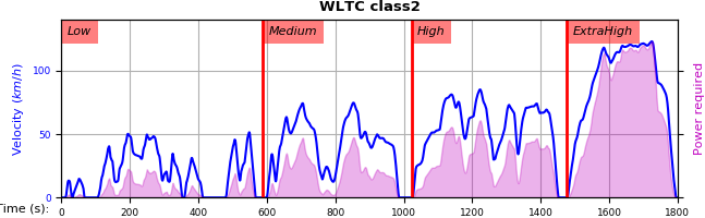
class2 |
V |
[0, 589] |
[589, 1022] |
[1022, 1477] |
[1477, 1800] |
VA0 |
[0, 588] |
[589, 1021] |
[1022, 1476] |
[1477, 1799] |
|
VA1 |
[1, 589] |
[590, 1022] |
[1023, 1477] |
[1478, 1800] |
|
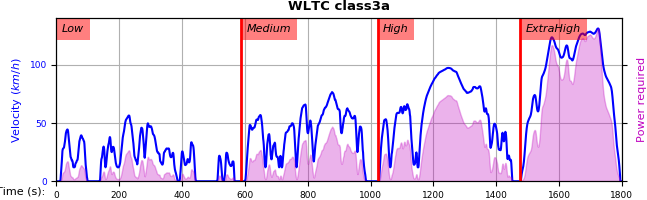
class3a |
V |
[0, 589] |
[589, 1022] |
[1022, 1477] |
[1477, 1800] |
VA0 |
[0, 588] |
[589, 1021] |
[1022, 1476] |
[1477, 1799] |
|
VA1 |
[1, 589] |
[590, 1022] |
[1023, 1477] |
[1478, 1800] |
|
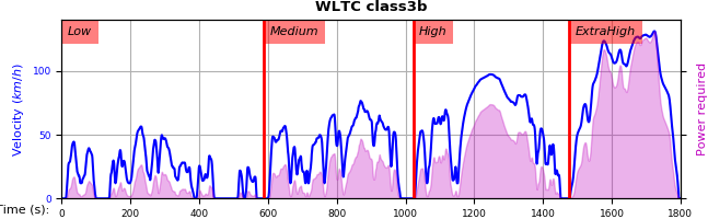
class3b |
V |
[0, 589] |
[589, 1022] |
[1022, 1477] |
[1477, 1800] |
VA0 |
[0, 588] |
[589, 1021] |
[1022, 1476] |
[1477, 1799] |
|
VA1 |
[1, 589] |
[590, 1022] |
[1023, 1477] |
[1478, 1800] |
6.1.1.7. Checksums
The
crc_velocity()function has been specially crafted to consume series of floats with 2-digits precision (v_decimals) denoting Velocity-traces, and spitting out a hexadecimal string, the CRC, without neglecting any zeros(0) in the trace.The checksums for all Phases (the problem) are reported by
cycle_checksums(), and the the table below is constructed. The original checksums of the GTR are also included in the final 2 columns.Based on this table of CRCs, the
identify_cycle_v_crc()function tries to match and identify any given Velocity-trace:
CRC32 |
SUM |
|||||||
|---|---|---|---|---|---|---|---|---|
by_phase |
cumulative |
by_phase |
cumulative |
|||||
phasing⇨ phase⇩ |
V |
VA0 |
VA1 |
V |
VA0 |
VA1 |
V |
V |
class1 |
||||||||
phase1 |
9840 |
4438 |
97DB |
9840 |
4438 |
97DB |
11988.4 |
11988.4 |
phase2 |
8C34 |
8C8D |
D9E8 |
DCF2 |
090B |
4295 |
17162.8 |
29151.2 |
phase3 |
9840 |
4438 |
97DB |
6D1D |
4691 |
F523 |
11988.4 |
41139.6 |
class2 |
||||||||
phase1 |
8591 |
CDD1 |
8A0A |
8591 |
CDD1 |
8A0A |
11162.2 |
11162.2 |
phase2 |
312D |
391A |
64F1 |
A010 |
606E |
3E77 |
17054.3 |
28216.5 |
phase3 |
81CD |
E29E |
9560 |
28FB |
9261 |
D162 |
24450.6 |
52667.1 |
phase4 |
8994 |
0D25 |
2181 |
474B |
262A |
F70F |
28869.8 |
81536.9 |
class3a |
||||||||
phase1 |
48E5 |
910C |
477E |
48E5 |
910C |
477E |
11140.3 |
11140.3 |
phase2 |
1494 |
D93B |
4148 |
403D |
2487 |
DE5A |
16995.7 |
28136.0 |
phase3 |
8B3B |
9887 |
9F96 |
D770 |
3F67 |
2EE9 |
25646.0 |
53782.0 |
phase4 |
F962 |
1A0A |
5177 |
9BCE |
9853 |
2B8A |
29714.9 |
83496.9 |
class3b |
||||||||
phase1 |
48E5 |
910C |
477E |
48E5 |
910C |
477E |
11140.3 |
11140.3 |
phase2 |
AF1D |
E501 |
FAC1 |
FBB4 |
18BD |
65D3 |
17121.2 |
28261.5 |
phase3 |
15F6 |
A779 |
015B |
43BC |
B997 |
BA25 |
25782.2 |
54043.7 |
phase4 |
F962 |
1A0A |
5177 |
639B |
0B7A |
D3DF |
29714.9 |
83758.6 |
… where if a some cycle-phase is identified as:
V phasing, it contains all samples;
VA0 phasing, it lacks -1 sample from the end;
VA1 phasing, it lacks -1 sample from the start.
6.1.1.8. Practical example
For instance, let’s identify the V-trace of class1’s full cycle:
>>> from wltp.datamodel import get_class_v_cycle  as wltc
>>> from wltp.cycles import identify_cycle_v as crc
>>> V = wltc("class1")
>>> crc(V)            # full cycle
('class1', None, 'V')
>>> crc(V[:-1])       # -1 (last) sample
('class1', None, 'VA0')
The crc() function returns a 3-tuple:
(i-class, i-phase, i-kind):
When
i-phaseis None, the trace was a full-cycle.
Now let’s identify the phases of “Access-DB”:
>>> crc(V[:590])      # AccDB phase1 respects GTR
('class1', 'phase-1', 'V')
>>> crc(V[590:1023])  # AccDB phase2 has -1 (first) sample
('class1', 'phase-2', 'VA1')
>>> crc(V[:1023])     # cumulative AccDB phase2 respects GTR
('class1', 'PHASE-2', 'V')
When
i-phaseis CAPITALIZED, the trace was cumulative.Phase2 is missing -1 sample from the start (
i-kind == VA1).
>>> crc(V[1023:])     # AccDB phase3
('class1', 'phase-1', 'VA1')
Phase3 was identified again as phase1, since they are identical.
Finally, clipping both samples from start & end, matches no CRC:
>>> crc(V[1:-1])
(None, None, None)
To be note, all cases above would have had identical CUMSUM (GTR’s) CRCs.